How To Remove Data Table In Excel Chart
Click on the small arrow next to the needed column name go to Filter by Color and pick the correct cell color. Remove the data table from your chart.

How To Format Data Table Numbers In Chart In Excel
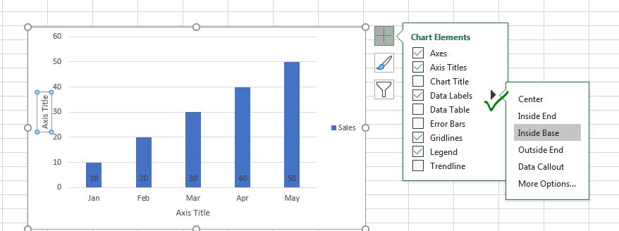
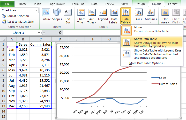
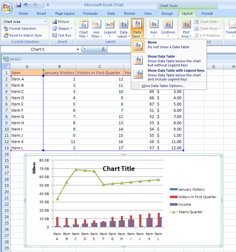
To show a data table point to Data Table and select the arrow next to it and then select a display option.
How to remove data table in excel chart. In excel in the chart tools group there is a function to add the data table to the chart. Make the background of your chart area No Fill so its transparent. Below are the steps to keep the Pivot table and remove the resulting data only.
Do one of the following. You wont find a delete table command in Excel. Click on the Analyze tab in the ribbon.
Make a new table on the worksheet that points via formulas to the range that the chart is made from. To clear the format from the table highlight or click in the table you wish to remove the formatting from. For example this sheet contains a table showing the busiest world airports.
This is a contextual tab that appears only when you have selected any cell in the Pivot Table. In the Actions group click on Clear option. Remove data labels from a chart.
Options include a choice not to show a data table show a data table but not show a chart legend or to show a data table and include the chart legend. This should bring you to the edit data point screen. Then select no border and no fill.
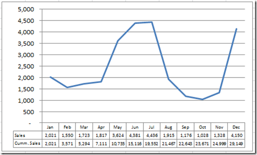
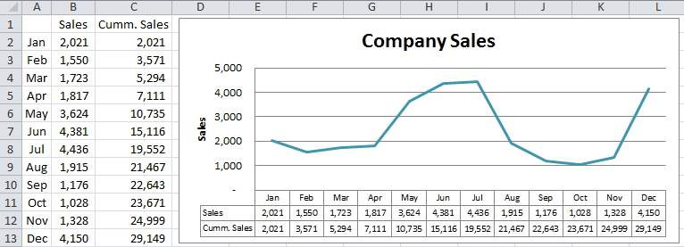
Note that the Table Design tab of the ribbon is a contextual tab and will only be visible when you are clicked in an Excel data table. In the example above the top chart includes blank cells which results in gaps in the plotted lines. Any changes to the cells of the data would change the chart as ex.
Click the chart from which you want to remove data labels. Now when the chart is selected the data range selector will. On the Design tab in the Chart Layouts group click Add Chart Element choose Data Labels and then click None.
Create a copy of the data set below the chart the chart must be in a worksheet not on a chart sheet Arrange the data set below the chart like you want to show it. Click OK and see all highlighted cells on top. In Excel 2013 click Design Add Chart Element Data Table to select With Legend Keys or No Legend Keys.
A cell in the table must be selected for the Design tab to be visible. In the Format Cells dialog click Number Number and then in the right section specify 2 in the Decimal places text box and check Use 1000 separator option. Hello youll have to fake it.
This displays the Table Tools adding the Design tab. Select format as table from the styles section. Resize the chart area to include the cells below it set the chart background to no fill and.
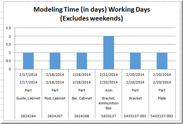
The data includes weekends but Pam doesnt want the weekend data included in the chart. If a table sits alone on a worksheet the fastest way is to delete the sheet. Click Chart Tools Layout Labels Data Table.
Select the filtered colored cells right-click on them and pick the Delete Row option from the menu. Make sure youre working on the home tab on excels ribbon and click on format as table and choose a style theme to convert your data to a table. This displays the Chart Tools adding the Design and Format tabs.
Removing 1 Item from the Data Table Below a Chart. Ive also changed the axis layout so you dont have to turn your head to read them which is always a nice touch. In other words she wants them displayed in the data table but not in the chart.
Right-click left-click right-click left-click. When you make a chart out of a table of data that chart is linked to the range of cells. How to remove whitespace on chart between columns and data table.
In excel in the chart tools group there is a function to add the data table to the chart. I dont want to include the quizzes in the chart but I can easily remove with the chart filter. If you have blank cells in a data table and want to plot a line chart with a continuous line without any gaps then you can replace the blanks with NAs using an IF statement see syntax below.
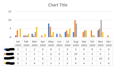
For example here I can select the chart then drag the data selector to include all 3 tests and the 2 quizzes. Right-click Excel 2007 or double click Excel 2010 the axis to open the Format Axis dialog box Axis Options Text Axis. For the second chart you need to reduce the axis X maximum value since there is no value more than 10 in your chart.
In those formulas use if statements to toggle the values onoff based on whatever logic you are using to hideshow. Click on Clear at the bottom of. The trick here is to first include all data then use the chart filter to remove the series you dont want.
Click OK to close the dialog then the original data and the data table numbers in the chart are changed at the same time. For the first char you need to select the chart and resize the columns area you might need to remove the chart title or move it somewhere else. Now your chart skips the missing dates see below.
Now the data table is added in the chart. In the lower chart the NA. To completely remove an Excel table and all associated data youll want to delete all associated rows and columns.
Show or hide a data table. Click Layout Data Table and select Show Data Table or Show Data Table with Legend Keys option as you need. Make sure youre working on the home tab on excels ribbon and click on format as table and choose a style theme to convert your data to a table.
To successfully complete this procedure you must have created an Excel table in your worksheet. Select format as table from the styles section. To hide the data table uncheck the Data Table option.
Audio Accessories Computers Laptops Computer Accessories Game Consoles Gifts Networking Phones Smart Home Software Tablets Toys Games TVs Wearables News Phones Internet Security Computers Smart Home Home Theater Software Apps Social Media Streaming Gaming Electric Vehicles Streaming WFH. Go to the Data tab in Excel and click on the Filter icon. Click anywhere in the table.
She knows that she could hide the rows and they would be excluded from the chart but she still needs the hidden rows to be displayed in the table. Select any cell in the Pivot Table. Make a Data Table.
Click anywhere on the chart you want to modify. Type the different percentages in column a. In the Ribbon select Table Design Table Styles and then click on the little down arrow at the bottom right hand corner of the group.
Just click the filter icon and uncheck quiz 1 and quiz 2. On the Design tab in the Tools group click Convert to Range. Below I use a checkbox.
On the errant data point in the graph. Select a chart and then select the plus sign to the top right.
How To Add And Remove Chart Elements In Excel
How To Add A Line To An Excel Chart Data Table And Not To The Excel Graph Excel Dashboard Templates
Show Or Hide A Chart Data Table Chart Data Chart Microsoft Office Excel 2007 Tutorial
How To Add A Line To An Excel Chart Data Table And Not To The Excel Graph Excel Dashboard Templates
How To Add A Line To An Excel Chart Data Table And Not To The Excel Graph Excel Dashboard Templates
How To Remove Whitespace On Chart Between Columns And Data Table Microsoft Tech Community


Excel Tutorial How To Add And Remove Data Series
How To Fake An Excel Chart Data Table With This Trick
How To Remove Whitespace On Chart Between Columns And Data Table Microsoft Tech Community
Post a Comment for "How To Remove Data Table In Excel Chart"